4. Time Series Concepts#
Let’s dive deeper into each of the topics: What is a time series, types of time series data, and applications of time series analysis, with more detailed explanations and example code where applicable.
4.1 What is a Time Series?#
A time series is a sequence of data points collected or recorded at specific time intervals. Each data point is associated with a timestamp, indicating when the observation was made. Time series data is typically collected in chronological order, making it suitable for analyzing and forecasting trends and patterns over time.
Time series data represents observations made sequentially through time. The field of time series analysis combined with AI offers numerous opportunities for extracting insights, modeling, prediction, and decision-making.
Here’s a comprehensive list of things you can do with time series information using AI:
Forecasting:
Short-Term Forecasts: Predicting values in the near future based on historical data (e.g., stock prices for the next week).
Long-Term Forecasts: Predicting values over longer time horizons (e.g., yearly sales projections).
Anomaly Detection:
Identifying unusual patterns that do not conform to expected behavior (e.g., spikes in website traffic or detecting fraud in credit card transactions).
Trend Analysis:
Discovering underlying trends in the data (e.g., increasing or decreasing sales, seasonal variations).
Seasonality Detection:
Identifying recurring short-term patterns at fixed intervals, such as hourly, daily, or yearly patterns.
Cyclical Patterns:
Identifying longer-term patterns that aren’t fixed (e.g., economic cycles).
Decomposition:
Breaking down a time series into its constituent components: trend, seasonality, and residual.
Classification:
Categorizing time series data into distinct classes or labels based on patterns (e.g., classifying machine operating modes based on sensor readings).
Clustering:
Grouping time series with similar patterns (e.g., customer purchase patterns).
Feature Extraction:
Extracting meaningful features from time series for further analysis, like Fourier transforms or wavelet coefficients.
Change Point Detection:
Detecting points in time where the statistical properties of the series change (e.g., detecting system changes or regime switches).
Fill Missing Values:
Using methods like interpolation, statistical imputation, or deep learning to fill in missing or corrupted time series data.
Causal Impact Analysis:
Evaluating the impact of an event on a time series (e.g., the effect of a marketing campaign on sales).
Time Series Segmentation:
Dividing a time series into meaningful segments or regimes (e.g., separating a long ECG signal into individual heartbeats).
Dynamic Time Warping (DTW):
Measuring similarity between two temporal sequences which may vary in speed (e.g., comparing speech patterns).
Cross-Correlation Analysis:
Evaluating the relationship between two or more time series (e.g., understanding the relationship between stock prices of two companies).
Embedding and Dimensionality Reduction:
Techniques like UMAP or t-SNE to visualize high-dimensional time series data in lower-dimensional space.
Transfer Learning:
Leveraging pre-trained models on one time series task and adapting it for another similar task.
Multivariate Time Series Analysis:
Handling and analyzing multiple time series simultaneously (e.g., forecasting stock prices using multiple related indicators).
Time Series Generative Models:
Generating new, synthetic time series data that resembles the original data, using methods like Generative Adversarial Networks (GANs).
Reinforcement Learning for Time Series:
Designing strategies for decision-making over time, for example, in stock trading.
Tools & Frameworks:
Traditional statistical models like ARIMA, Exponential Smoothing.
Machine Learning models such as Random Forests, SVMs, and Gradient Boosting tailored for time series.
Deep Learning models like Long Short-Term Memory (LSTM) networks, GRUs, and 1D CNNs.
Libraries like Prophet (by Facebook), TensorFlow, PyTorch, and scikit-learn.
When working with time series data using AI, it’s important to consider aspects like stationarity, autocorrelation, lag variables, and more. Proper preprocessing and understanding of the data are key to effective modeling and analysis.
4.2 Applications of Time Series Analysis#
Time series analysis has a wide range of applications across various domains, including:
Economics: Analyzing economic indicators like GDP, inflation rates, and unemployment data for forecasting and policy-making.
Finance: Predicting stock prices, analyzing financial market data, and risk assessment using techniques like GARCH models.
Meteorology: Forecasting weather patterns, temperature, precipitation, and climate change modeling.
Healthcare: Monitoring and analyzing patient data, disease outbreaks, medical device telemetry, and drug development.
Manufacturing: Quality control, demand forecasting, and production optimization to reduce costs and improve efficiency.
Marketing: Analyzing sales data, customer behavior, and campaign effectiveness for targeted marketing strategies.
Environmental Science: Studying environmental data such as air quality, pollution levels, and ecological trends.
Energy: Predicting energy demand, optimizing energy production, and forecasting renewable energy generation.
Anomaly Detection: Identifying unusual patterns or anomalies in data for fraud detection, fault detection, and network security.
Social Sciences: Analyzing social data over time, such as population demographics, social media trends, and sentiment analysis.
These are just a few examples of the many applications of time series analysis. Depending on your domain or specific problem, you can apply various time series modeling techniques and statistical methods to gain insights and make predictions.
4.3 Types of Time Series Data#
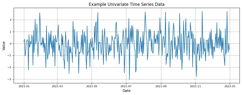
Univariate Time Series: This type contains a single variable recorded over time, such as temperature or stock prices. It involves the analysis of a single data series.
Applications of univariate time series analysis include:
Economic forecasting: Predicting future economic trends based on past trends in key economic indicators such as inflation rates and GDP.
Financial forecasting: Predicting future trends in financial markets based on historical data.
Weather forecasting: Predicting future weather patterns based on historical weather data.
Sales forecasting: Predicting future sales of a product based on historical sales data.
import pandas as pd
import numpy as np
import matplotlib.pyplot as plt

# Generate a simple time series dataset
date_rng = pd.date_range(start='2021-01-01', end='2021-12-31', freq='D')
data = np.random.randn(len(date_rng))  # Random data for illustration
ts = pd.Series(data, index=date_rng)

# Plot the time series data
plt.figure(figsize=(10, 4))  # Adjust the figure size as per your preference
plt.plot(ts)
plt.title("Example Univariate Time Series Data", fontsize=12)  # Adjust title font size
plt.xlabel("Date", fontsize=10)  # Adjust x-axis label font size
plt.ylabel("Value", fontsize=10)  # Adjust y-axis label font size
plt.grid(True)

# Adjust tick label font size for both x and y axes
plt.xticks(fontsize=8)
plt.yticks(fontsize=8)

plt.tight_layout()  # Ensure all elements fit within the figure
plt.show()
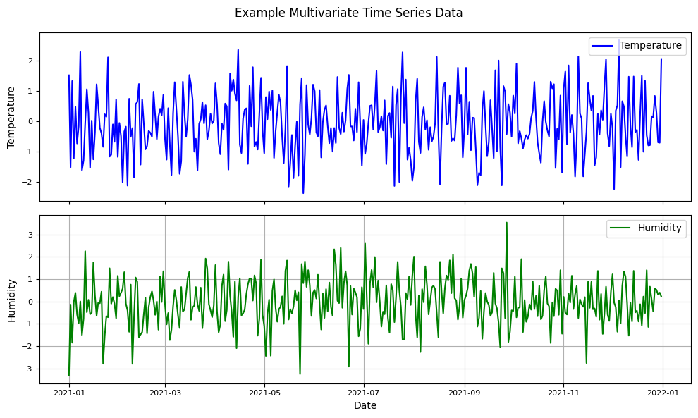
Multivariate Time Series: In this type, multiple variables are recorded over time. For example, you might have time series data for temperature, humidity, and wind speed over the same time period.
Applications of multivariate time series analysis include:
Traffic forecasting: Predicting future traffic patterns based on weather, time of day, and other factors.
Climate modeling: Modeling how different factors such as temperature, precipitation, and CO2 emissions impact global climate patterns.
Marketing analytics: Analyzing the impact of multiple marketing channels on sales and customer behavior.
Supply chain optimization: Optimizing the supply chain by analyzing multiple variables such as production capacity, shipping times, and inventory levels.
In the field of time-series machine learning, it is important to differentiate between univariate and multivariate datasets. Univariate algorithms are only capable of working with a single feature, while multivariate algorithms are able to work with many features.
Traditionally, classical modeling techniques have focused on univariate datasets and their applications. These datasets consist of cases that have a single series and a class label, and they are often the only ones available for analysis.
However, in practice, multivariate time-series datasets are much more common than univariate ones. These datasets have multiple feature dimensions and are found in many real-life applications, such as human activity recognition, diagnoses based on an electrocardiogram (ECG), electroencephalogram (EEG), magnetoencephalography (MEG), and systems monitoring.
import pandas as pd
import numpy as np
import matplotlib.pyplot as plt

# Generate multivariate time series data
date_rng = pd.date_range(start='2021-01-01', end='2021-12-31', freq='D')
data = np.random.randn(len(date_rng), 2)  # Simulated data for two variables
df_multivariate = pd.DataFrame(data, index=date_rng, columns=['Temperature', 'Humidity'])

# Create a figure with two subplots
fig, axs = plt.subplots(2, 1, figsize=(10, 6), sharex=True)  # Adjust the figure size

# Plot Temperature in the first subplot
axs[0].plot(df_multivariate.index, df_multivariate['Temperature'], label='Temperature', color='blue')
axs[0].set_ylabel("Temperature", fontsize=10)  # Adjust font size
axs[0].legend()
plt.grid(True)

# Plot Humidity in the second subplot
axs[1].plot(df_multivariate.index, df_multivariate['Humidity'], label='Humidity', color='green')
axs[1].set_xlabel("Date", fontsize=10)  # Adjust font size
axs[1].set_ylabel("Humidity", fontsize=10)  # Adjust font size
axs[1].legend()

# Set a common title for both subplots
plt.suptitle("Example Multivariate Time Series Data", fontsize=12)  # Adjust title font size
plt.grid(True)

# Adjust tick label font size for both subplots
for ax in axs:
    ax.tick_params(axis='both', labelsize=8)

plt.tight_layout()  # Ensure all elements fit within the figure
plt.show()
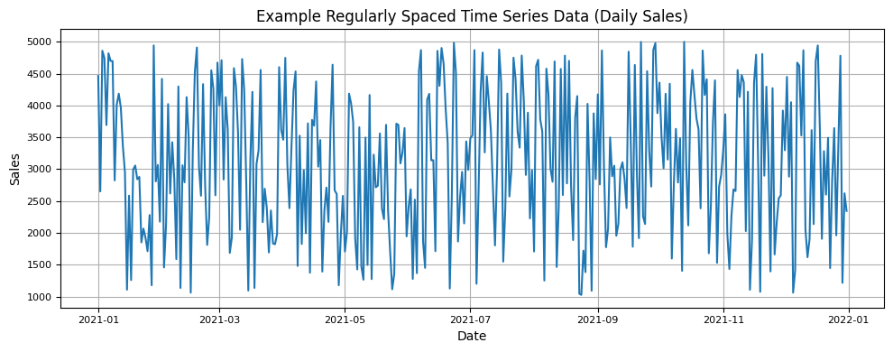
Regularly Spaced Time Series: Data points are collected at fixed, regular intervals, such as hourly, daily, or monthly.
import pandas as pd
import numpy as np
import matplotlib.pyplot as plt

# Generate regularly spaced time series data (daily sales)
date_rng = pd.date_range(start='2021-01-01', end='2021-12-31', freq='D')
sales_data = np.random.randint(1000, 5000, size=len(date_rng))  # Simulated daily sales data
sales_ts = pd.Series(sales_data, index=date_rng)

# Plot the regularly spaced time series data
plt.figure(figsize=(10, 4))  # Adjust the figure size as per your preference
plt.plot(sales_ts)
plt.title("Example Regularly Spaced Time Series Data (Daily Sales)", fontsize=12)  # Adjust title font size
plt.xlabel("Date", fontsize=10)  # Adjust x-axis label font size
plt.ylabel("Sales", fontsize=10)  # Adjust y-axis label font size
plt.grid(True)

# Adjust tick label font size for both x and y axes
plt.xticks(fontsize=8)
plt.yticks(fontsize=8)

plt.tight_layout()  # Ensure all elements fit within the figure
plt.show()
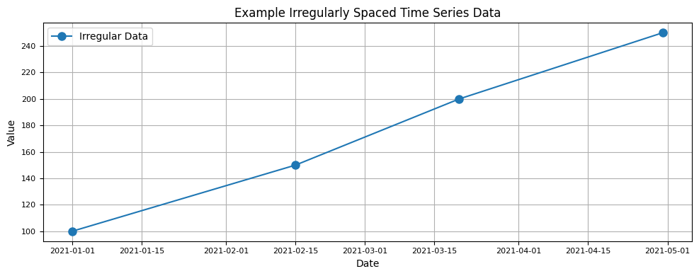
Irregularly Spaced Time Series: Data points are collected at irregular intervals, and handling missing data or irregular time gaps becomes necessary.
import pandas as pd
import matplotlib.pyplot as plt

# Example: Irregularly spaced time series data
dates = ['2021-01-01', '2021-02-15', '2021-03-20', '2021-04-30']
values = [100, 150, 200, 250]
irregular_ts = pd.Series(values, index=pd.to_datetime(dates))

# Plot the irregularly spaced time series data
plt.figure(figsize=(10, 4))  # Adjust the figure size as per your preference
plt.plot(irregular_ts.index, irregular_ts.values, 'o-', markersize=8, label='Irregular Data')
plt.title("Example Irregularly Spaced Time Series Data", fontsize=12)  # Adjust title font size
plt.xlabel("Date", fontsize=10)  # Adjust x-axis label font size
plt.ylabel("Value", fontsize=10)  # Adjust y-axis label font size
plt.legend()
plt.grid(True)

# Adjust tick label font size for both x and y axes
plt.xticks(fontsize=8)
plt.yticks(fontsize=8)

plt.tight_layout()  # Ensure all elements fit within the figure
plt.show()
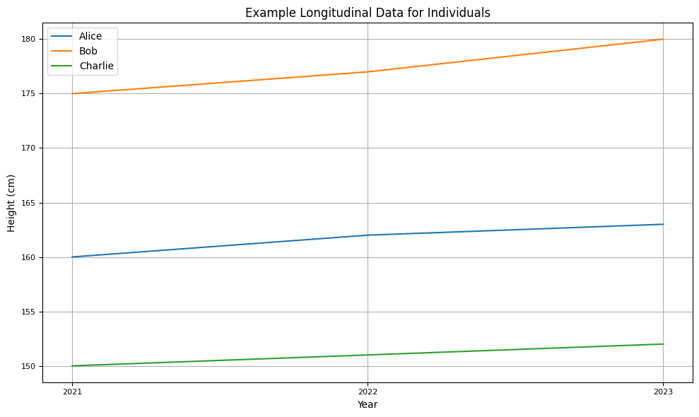
Longitudinal Data: Time series data recorded for the same entities (e.g., individuals or companies) at multiple time points. It’s often used in medical and social sciences research.
import pandas as pd
import matplotlib.pyplot as plt

# Example: Longitudinal data for individuals
individuals = ['Alice', 'Bob', 'Charlie']
data = {
    'Alice': [160, 162, 163],
    'Bob': [175, 177, 180],
    'Charlie': [150, 151, 152]
}
df_longitudinal = pd.DataFrame(data, index=[2021, 2022, 2023])

# Plot longitudinal data for individuals
plt.figure(figsize=(10, 6))  # Adjust the figure size as per your preference
for person in individuals:
    plt.plot(df_longitudinal.index, df_longitudinal[person], label=person)

plt.title("Example Longitudinal Data for Individuals", fontsize=12)  # Adjust title font size
plt.xlabel("Year", fontsize=10)  # Adjust x-axis label font size
plt.ylabel("Height (cm)", fontsize=10)  # Adjust y-axis label font size
plt.legend()
plt.grid(True)

# Adjust tick label font size for both x and y axes
plt.xticks(df_longitudinal.index, fontsize=8)
plt.yticks(fontsize=8)

plt.tight_layout()  # Ensure all elements fit within the figure
plt.show()
4.4 Time Series Components#
Time series data is a sequence of observations collected at successive points in time, usually at regular intervals. There are three primary components in most time series datasets:
Trend: The long-term movement in the data. It could be upward, downward, or flat.
Seasonality: Patterns that repeat at known regular intervals. This is usually observed in data like retail sales, which may spike during holiday seasons.
Noise: Random fluctuations in data that don’t have any pattern.
Example: Monthly sales data for an ice cream shop may have an upward trend in summer (because of increased consumption) and downward in winter. The spikes in sales during weekends might be the seasonality, and any random events causing spikes or drops would be considered noise.
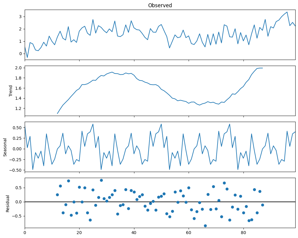
4.5 Time Series Decomposition#
This is the process of breaking down a time series into its constituent components: trend, seasonality, and noise.
Python’s statsmodels library provides a method for decomposing time series.
Example code:
import pandas as pd
import numpy as np
import matplotlib.pyplot as plt
from statsmodels.tsa.seasonal import seasonal_decompose

# Set the figure size and font size
plt.rcParams['figure.figsize'] = (10, 8)  # width, height in inches
plt.rcParams['font.size'] = 10  # Decrease the font size

# Generate sample time series data
time = np.linspace(0, 2 * np.pi, 100)
trend = time * 0.5
seasonality = np.sin(time)
noise = np.random.normal(0, 0.5, 100)
timeseries = trend + seasonality + noise

# Decompose the time series
result = seasonal_decompose(timeseries, model='additive', period=25)

# Plot the decomposed time series
result.plot()
plt.tight_layout()  # Adjust subplot parameters to give specified padding
plt.show()
4.6 Stationarity and Non-stationarity#
Stationarity: A time series is said to be stationary if its statistical properties (like mean, variance) remain constant over time. This is important because most time series forecasting methods assume that the series is stationary.
Non-stationarity: If the series has varying mean or variance over time.
To test for stationarity, one popular method is the Augmented Dickey-Fuller (ADF) test. A p-value smaller than a threshold (e.g., 0.05) suggests that the series is stationary.
Example code:
from statsmodels.tsa.stattools import adfuller

# Conduct ADF test
result = adfuller(timeseries)

print('ADF Statistic:', result[0])
print('p-value:', result[1])

if result[1] < 0.05:
    print("The series is likely stationary.")
else:
    print("The series is likely non-stationary.")
ADF Statistic: -3.5211291325488783
p-value: 0.007460747736202724
The series is likely stationary.